If you're a microbial ecologist and you haven't used phyloseq, put away your vintage scarf and thick-rimmed glasses because you are not hip. phyloseq is the nexus of all that is good in the universe. In this post we'll look at one of the greatest phyloseq functions, psmelt. psmelt combines your sample info, OTU counts, and taxonomic annotations into a single dataframe where every row represents an OTU-sample combination. Hhhhwhat!?! Amazing, I know. From this omnipotent dataframe you can do anything. So, how do we use psmelt? And can we re-create psmelt with dplyr and tidyr?
Let's start by bringing in some R packages and loading the rmagic extension for IPython.
%load_ext rpy2.ipython
%%R
library(phyloseq)
library(dplyr); library(tidyr)
library(magrittr)
library(ggplot2)
I'm going to use data from a paper we recently submitted. See the pre-print here if you're interested. A typical microbiome data set consists of three tables:
- A table of sample information.
- A table of OTU counts in the samples.
- A table of taxonomic info for each OTU.
In this example the OTU counts and taxonomic info are combined in a json biom formatted table. We have the sample information in a QIIME formatted sample metadata table. Don't get bogged down in the file formats, however. They're just tables and you can get tables into R easily. Focus on the concepts and what information you need to do an analysis.
We'll write a quick function to handle the QIIME formatted sample data table (note how we're just using the base R read.table function) and we'll use the import_biom function from phyloseq to import our OTU counts and OTU taxonomic annotations. We'll combine all the info into a phyloseq object.
%%R
read.qiime = function(fn) {
    read.table(fn, sep = "\t", comment = "", header = TRUE, stringsAsFactors = FALSE) %>%
    rename(SampleID = X.SampleID) %>%
    {rownames(.) = .$SampleID; .} %>%
    data.frame %>% sample_data
}

physeq = import_biom("data/otu_table_wtax.biom")
sample_data(physeq) = read.qiime("data/sample_data_combined_qiime_format.tsv")
physeq
Great! Now let's melt all that information into an all-powerful, all-knowing, benevolent dataframe. (Evil laugh)
%%R
mdf = psmelt(physeq)
mdf %>% select(OTU, SampleID, Abundance) %>% head
To keep this post short, I won't demonstrate where you can go from a melted phyloseq object. Suffice to say that you can go anywhere with your melted phyloseq object/dataframe. Think of it like a magic carpet.
With really big OTU tables, melting can take a long time...
%%R
system.time(psmelt(physeq))
It takes about 30-ish seconds with our example phyloseq object with the psmelt function. I wonder how fast dplyr + tidyr can melt our phyloseq object?
Let's re-create the psmelt function with dplyr + tidyr.
We need to,
- get our tables (sample data, OTU counts, taxonomy),
- combine our taxonomic info with our OTU counts,
- gather this combined table into a long form version, and
- add in the sample data.
%%R
psmelt.dplyr = function(physeq) {
    sd = data.frame(sample_data(physeq))
    TT = data.frame(tax_table(physeq)) %>% add_rownames("OTU")
    otu.table = data.frame(otu_table(physeq), check.names = FALSE) %>% add_rownames("OTU")
    otu.table %>%
        left_join(TT) %>%
        gather_("SampleID", "Abundance", setdiff(colnames(otu.table), "OTU")) %>%
        left_join(sd)
}
%%R
mdf.dplyr = psmelt.dplyr(physeq)
mdf.dplyr %>% select(OTU, SampleID, Abundance) %>% head
...and let's see how fast it is.
%%R
system.time(psmelt.dplyr(physeq))
Wow. Roughly an order of magnitude faster. dplyr and tidyr are so great. And look at that syntax!
I shold note that I'm using phyloseq version 1.9.15 in this demo.
The psmelt function is so useful (and much more rigorous/fool-proof than our quick dplyr/tidyr version) but if you have a huge phyloseq object that takes forever to melt, try dplyr + tidyr.
Let's do one quick example from the melted phyloseq object to give you a taste of how useful it is. Let's say we want to make phylum level stacked bar charts for all the studies in the example data. Here's how you might do it from the melted phyloseq object.
%%R -w 1200
d = mdf.dplyr %>%
    group_by(SampleID, Rank2) %>%
    filter(Abundance > 0) %>%
    summarize(rank2.abund = sum(Abundance), study = first(study)) %>%
    mutate(relative.abundance = rank2.abund / sum(rank2.abund))

p = ggplot(d, aes(x = SampleID, y = relative.abundance, fill = Rank2)) +
    facet_grid(.~study, drop = TRUE, space = "free", scales = "free") +
    geom_bar(stat = "identity", width = 0.85) +
    theme_bw() + theme(axis.text.x = element_blank(), legend.position = "none", strip.background = element_blank())
p
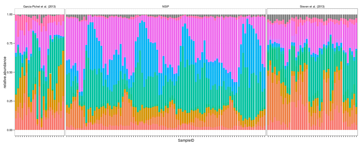
Snap.
%%R
pckgs  = lapply(names(sessionInfo()$otherPkgs), packageVersion)
names(pckgs) = names(sessionInfo()$otherPkgs)
data.frame(pckgs)