%load_ext rpy2.ipythonMaking trees in the Jupyter notebook (part 1 - IToL)
Let’s extend the previous post by scraping the CAZy website for accession numbers from genes in the glycoside hydrolase 5 (GH5) family. Then we can build a phylogenetic tree from these sequences and visualize how well the EC activities correspond to the phylogeny.
Unfortunately the CAZy website spreads the information we need across multiple pages in tables that are not easily parsed. Luckily we have rvest. Let’s start by loading the libraries we’ll use.
%%R
library(rvest)
library(magrittr)
library(plyr); library(dplyr)
library(rentrez)
library(ggplot2)
library(rwantshue)
CAZy distinguishes between genes that have been biochemically characterized and those that haven’t. For this analysis we’ll stick the characterized genes. This is the website that we’ll be scraping:
www.cazy.org/GH5_characterized.html
All we really need is a table of accessions and corresponding EC numbers but we might as well grab some other information provided by CAZy such as the subfamily membership of each gene and the organism.
We’ll start by creating a session from the webpage above.
%%R
cazy = html_session("http://www.cazy.org/GH5_characterized.html")
We need to grab the links to the pages that contain continued sections for our table. I use Chrome’s inspector tools or the SelectorGadget to find the attributes and element data associated with the information I want to scrape. In this case, the webpage links we want are in span elements of the “pages” class. Each span element has a hyperlink tag (“a” below in html_nodes) and from that tag we want the value of the “href” attribute.
%%R
links = cazy %>% html_nodes("span.pages a") %>% html_attr("href")
links
[1] "GH5_characterized.html?debut_PRINC=100#pagination_PRINC"
[2] "GH5_characterized.html?debut_PRINC=200#pagination_PRINC"
[3] "GH5_characterized.html?debut_PRINC=300#pagination_PRINC"
[4] "GH5_characterized.html?debut_PRINC=400#pagination_PRINC"
[5] "GH5_characterized.html?debut_PRINC=500#pagination_PRINC"Let’s start by scraping the first page (the page we’re currently on).
The table has some rows that we don’t want (like the row that just points out the Domain of the organisms) which makes parsing this info a bit tricky. We need to scrub rows with the “royaume” class and rows with id “line_titre” (I think those are French words). So, to briefly summarize the command below, we’re grabbing rows (“tr”) from the table of class “listing” excluding rows of class “royaume” and id “line_titre”.
%%R
rows = cazy %>% html_nodes("table.listing tr:not(.royaume)[id!=line_titre]")
We’ll parse each row to get the accession, EC number, organism, and subfamily. I’m only grabbing the linked accession number. Some of the genes have multiple associated accession numbers but I think we’ll only need one. Also, I’m creating one row for each EC number so some of the genes will have two entries. I think I’ll eventually remove the genes with multiple EC activities from the tree but it might also be nice to point them out. Note how we use the extract2 function from magrittr to get the correct column.
%%R
get_data = function(row) {
    cols = row %>% html_nodes("td")
    ec = cols %>% extract2(2) %>% html_nodes("font.E") %>% html_text() %>% unlist
    organism = cols %>% extract2(3) %>% html_text(trim = TRUE)
    acc = cols %>% extract2(4) %>% html_nodes("a b") %>% html_text()
    if ( length(acc) == 0 )  {
        acc = cols %>% extract2(4) %>% html_text() %>% substr(1,10)
    }
    subf = cols %>% extract2(7) %>% html_text(trim = TRUE)
    data.frame(ec=ec, organism=organism, acc=acc, subf=subf)
}
And now we’ll ldply it into a handy dataframe.
%%R
df.pg1 = ldply(rows, get_data)
df.pg1 %>% head
ec organism acc subf
1 3.2.1.4 Desulfurococcaceae archaeon EBI-244 AEB53062.1
2 3.2.1.- Halorhabdus utahensis DSM 12940 ACV12553.1
3 3.2.1.4 Pyrococcus abyssi GE5 CAB49854.1 1
4 3.2.1.4 Pyrococcus horikoshii OT3 AAQ31833.1 1
5 3.2.1.78 Acidothermus cellulolyticus ABJ41262.1 7
6 3.2.1.4 Acidothermus cellulolyticus 11B ATCC 43068 AAA75477.1 1Now we need to do that for all the other pages of the table. This function uses jump_to to go to a link and extract the information we need with the same code as we had above. We can append our page 1 information with rbind and we’re ready to go.
%%R
get_df = function(link) {
    session = jump_to(cazy, link)
    rows = session %>% html_nodes("table.listing tr:not(.royaume)[id!=line_titre]")
    rows %>% head
    ldply(rows, get_data)
}

df.all = ldply(links, get_df) %>% rbind(df.pg1)
df.all %>% head
ec organism acc subf
1 3.2.1.78 Clostridium cellulovorans 743B ADL52789.1 7
2 3.2.1.78 Clostridium cellulovorans 743B AAF06110.2 17
3 3.2.1.4 Clostridium cellulovorans ATCC 35269 AAA23233.1 4
4 3.2.1.73 Clostridium cellulovorans ATCC 35269 AAA23233.1 4
5 3.2.1.8 Clostridium cellulovorans ATCC 35269 AAA23233.1 4
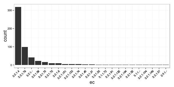
6 3.2.1.4 Clostridium cellulovorans ATCC 35269 AAD39739.1 4We now have all the information we need to make our tree in IToL that will give us a sense of how phylogenetically conserved the EC annotations are with phylogeny. But first let’s plot some counts of the different EC activities. There is clearly one predominant activity for this set of sequences.
%%R -h 300 -w 600
df.all %>%
    group_by(ec) %>%
    summarize(count = n()) %>% {
        xsort = arrange(., desc(count)) %>% extract2("ec")
        mutate(., ec = factor(ec, levels = xsort)) %>%
        ggplot(aes(x = ec, y = count)) +
            geom_bar(stat = "identity") +
            theme_bw() +
            theme(axis.text.x = element_text(angle = 45, hjust = 1),
                  axis.title = element_text(size = 16))
}%%R
df.all %>% write.csv("data/GH5_data.csv", row.names = FALSE, quote = FALSE)We should add one more bit of information to the dataframe, the colors for each EC number. We need to send this information to IToL. Below I’m using rwantshue to get a list of colors the same length as the number of observed EC numbers. We collect the colors for each EC number in a dataframe and then we can join that colors dataframe to our CAZy dataframe. We’ll also save the IToL information to a file. I am making what IToL refers to as a “colors definition” file. This file should include (in order) a column for the tip names on the tree (in our case this will be accessions), a column specifying what you want to color (“range” here see IToL website for details), the actual color, and the label (EC numbers in our case).
%%R
N = df.all$ec %>% unique %>% length
scheme <- iwanthue()
colors = scheme$hex(N, color_space = hcl_presets$intense)
col.df = data.frame(
    colors = colors,
    ec = df.all$ec %>% unique
)
df.all %>%
    left_join(col.df) %>%
    mutate(ctype = "range", label = ec) %>%
    select(acc, ctype, colors, label) %>%
    group_by(acc) %>% filter(row_number() == 1) %>% # just grab the first row for each seq.
                                                    # Some seqs have two EC numbers.
    write.table("data/color_defs.tsv", row.names = FALSE, col.names = FALSE, sep = "\t", quote = FALSE)
Here’s what that file looks like,
!head -n5 data/color_defs.tsvADL52789.1 range #4FB197 3.2.1.78
AAF06110.2 range #4FB197 3.2.1.78
AAA23233.1 range #CA55E1 3.2.1.4
AAD39739.1 range #CA55E1 3.2.1.4
BAA12826.1 range #CA55E1 3.2.1.4Great! Now on to building the tree…
We need to get the sequences first. Let’s use rentrez to query Genbank for our accessions.
%%R
accs = df.all$acc %>% as.character %>% unique
seqs = entrez_fetch(db="nucleotide", id=accs, rettype="fasta")
write(seqs, "data/GH5_characterized.fasta")!head -n3 data/GH5_characterized.fasta>gi|328834886|gb|AEB53062.1| putative glycoside hydrolase family 5 [Desulfurococcaceae archaeon EBI-244]
MKKVHIIAIVVIIAIAFALILARYYTMQRGYETVTPTTPPQQTTTTETTPVPTEAGTTTPITEATVTQPP
QTPTTPSPQTPTTPTALPTPSPTPTAPSATVTETTSPQTPTTTITTETTTTPAPQPQVVFLKLPEGEEPKI’m going to align these sequences with Muscle.
!muscle -in data/GH5_characterized.fasta -out data/GH5_characterized.aln.fasta!head -n5 data/GH5_characterized.aln.fasta>gi|190684977|gb|ACE82655.1| endo-1, 4-beta mannanase, man5C [Cellvibrio japonicus Ueda107]
------------------------------------------------------------
------------------------------------------------------------
------------------------------------------------------------
-------------------------------------------MKHLISPRILTGLFVIGOk, we’re going to switch into Python mode now as we have a look at this alignment. Also, we’ll use Python to talk to IToL. Let’s just plot gap frequency by position.
from skbio.alignment import Alignment
from skbio.sequence import DNA
import seaborn as sns
import matplotlib.pyplot as plt
import numpy as np
from itolapi import Itol, ItolExport
from IPython.display import Image
%matplotlib inline
aln = Alignment.read(file = "data/GH5_characterized.aln.fasta", format="fasta")Our alignment is a bit gappy as you can see below. There are quite a few positions with few characters.
gap_freq = [d["-"] for d in aln.position_frequencies()]
fig, ax = plt.subplots()
fig.set_size_inches([16, 3])
ax.plot(np.arange(len(gap_freq)), gap_freq)
ax.set_xlabel("Position")
ax.set_ylabel("Gap frequency")
Let’s make a gap frequency filter to remove columns with greater than 60% gaps.
keepers, = np.where(np.array(gap_freq)<=0.60)
aln_masked = aln.subalignment(positions_to_keep=keepers)
Ok, that looks better. We’ll use this filtered alignment to build the tree.
gap_freq2 = [d["-"] for d in aln_masked.position_frequencies()]
fig, ax = plt.subplots()
fig.set_size_inches([16, 3])
ax.plot(np.arange(len(gap_freq2)), gap_freq2)
ax.set_xlabel("Position")
ax.set_ylabel("Gap frequency")aln_masked.write("data/GH5_characterized.aln.masked.fasta", format="fasta")'data/GH5_characterized.aln.masked.fasta'!head -n2 data/GH5_characterized.aln.masked.fasta | cut -c1-100>gi|190684977|gb|ACE82655.1| endo-1, 4-beta mannanase, man5C [Cellvibrio japonicus Ueda107]
HLISPRILTGLFVIGLAPAWSSSVSSSGIIVGAQCNWYGPVCQSGASLPAPGNSVL-SGSSPEGNSWLSPYS-SKVMDGTASYAFAEATVPVTYQGQGDGI’m going to make the tree with FastTree. I’m doing a quick hack to make sure that the tips of our tree are just accession numbers and not the long identifiers returned from rentrez. The sed command just grabs the accession from each FASTA identifier line and scrubs the rest. I am using process substitution but you could just as easily write the scrubbed FASTA to a file and send it to FastTree.
!head -n6 data/GH5_characterized.aln.masked.fasta | sed '/^>/ s/.*|.*|.*|\(.*\)|.*/>\1/' | cut -c 1-80 #for example...>ACE82655.1
HLISPRILTGLFVIGLAPAWSSSVSSSGIIVGAQCNWYGPVCQSGASLPAPGNSVL-SGSSPEGNSWLSPYS-SKVMDGT
>AFR99035.1
----MPPPPEVSPVTG-------------NPVSPHYIHS------STL-HFGRSLVLRGVN--EGFWFPLNLDDGSLARL
>BAG70961.1
MKAMTSVILPPVAAPALCLAAV---------WTTFNAVG------ANL-G-GW---LIDTTGAVDEWCGPVLEWITIDTL%%bash
FastTree <(sed '/^>/ s/.*|.*|.*|\(.*\)|.*/>\1/' data/GH5_characterized.aln.masked.fasta) > data/GH5.tree 2>/dev/nullCool, now we just need to upload the tree and the color definition file from above to IToL. There is a nice Python library to talk to IToL programatically called itolapi. We’re using that to upload our info. The itolapi page has all the documentation required to use it effectively.
itol_uploader = Itol.Itol()
itol_uploader.add_variable('treeFile', 'data/GH5.tree')
itol_uploader.add_variable('treeFormat', 'newick')
itol_uploader.add_variable('treeName', 'GH5')
itol_uploader.add_variable("colorDefinitionFile", "data/color_defs.tsv")
status = itol_uploader.upload()
itol_uploader.comm.upload_output
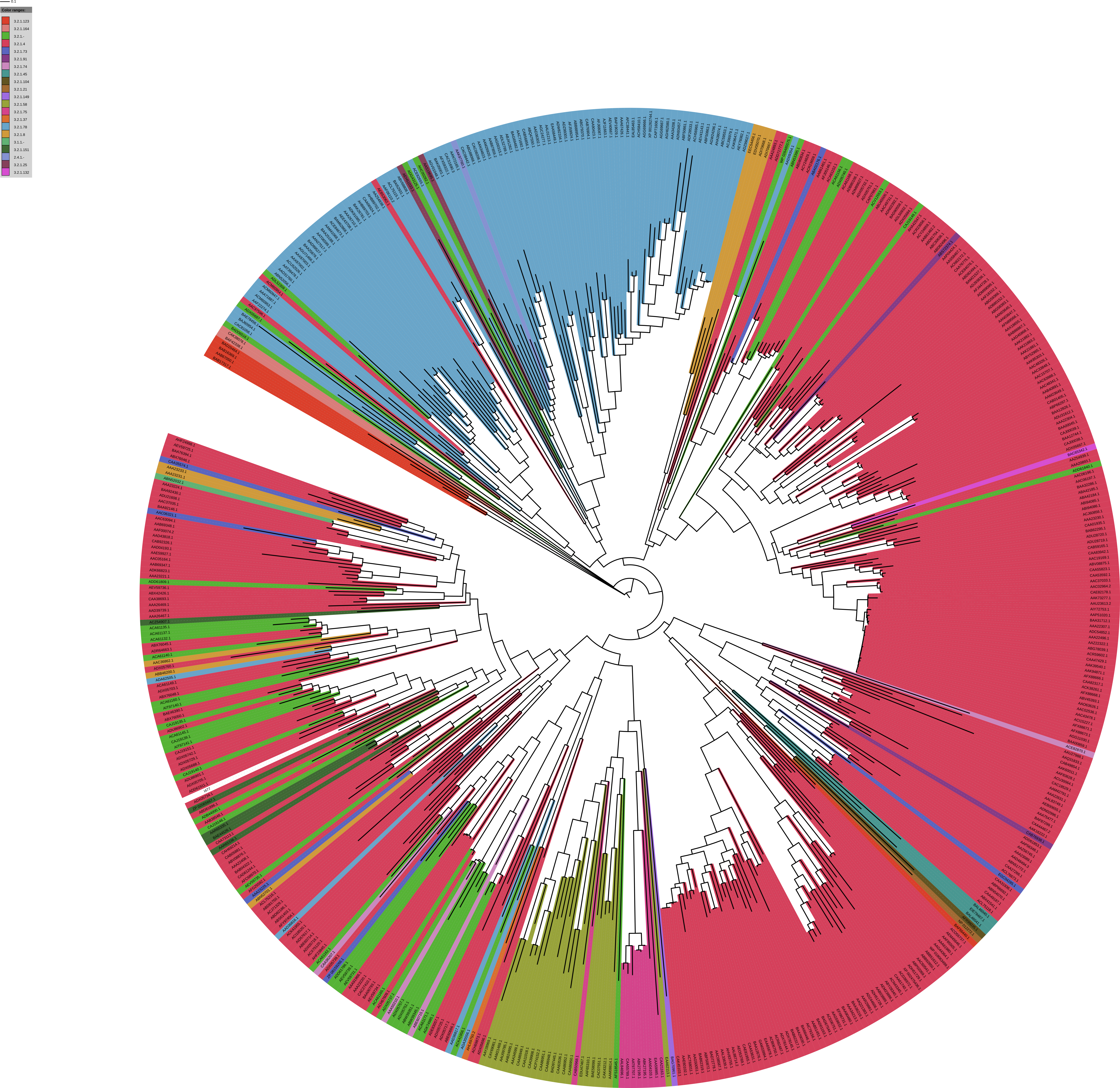
print itol_uploader.get_webpage()http://itol.embl.de/external.cgi?tree=128841252312946714389719820&restore_saved=1You can also use itolapi to download the tree but I don’t think the IToL API supports exporting trees with full clade coloring. I could be wrong but I really wanted the full clade coloring as opposed to just a ring of colors around the tree. Anyway, I had to manually visit IToL to export this visualization (frown).
So it looks like there’s some coherence to the EC numbers. The two main EC annotations do not appear to overlap much but the minor annotations are dispersed throughout in small groups.
You can explore this tree in IToL by visiting this page.
Disclaimer: I don’t want to go down the rabbit hole of finding all the inconsistencies in this CAZy table for this small example. There are most definitely some wonky rows in the information we scraped. I think the accessions are the least consistent field in CAZy and it’s tiresome to account for all the seemingly arbitrary little ways that rows can differ from the consensus. The moral of the story? Don’t make people scrape your webpage to get information!!! I don’t see why that table can’t be provided by the CAZy team as a nice CSV…


